Applications of Neural Networks to Music Generation

By Anna Mikhailova

Music generation, alternatively termed algorithmic composition, or music synthesis, is the process of generating music via an algorithm (i.e. some formal set of rules). Algorithmic music composition has been a part of the human experience for millennia – transcending cultures and continents. It ranges from any music that is generated without human interference – e.g. wind chimes – to music generated by intelligent systems. The application of neural networks to music generation poses particular interest due to the similarity between music composition and natural language structuring. A similar challenge to that of language is that any given instance of “music” can contain more than just one music unit (i.e. a note). It can consist of several notes together (a chord) and/or other qualities such as volume, much like language. The creation of “convincing” music, or music that sounds like it could be naturally produced by a human, is riddled with challenges. Although not all algorithmic music has aimed to produce human-like creations, that goal has been at the forefront of ongoing research.

A Brief History

In the absence of modern technology (pre-1700), the precursor to what we nowadays refer to as algorithmic music was automatic music – music arising from naturally, or automatically, occurring processes. Automatic music generation has allegedly been a human obsession since biblical times. Legend has it that King David hung a lyre above his bed to catch the wind at night, and thus produce music. These wind instruments, known as Aeolian harps have been found throughout history in China, Ethiopia, Greece, Indonesia, India, and Melanesia. Music generated by the wind exists to this day, in the form of wind chimes, which first appeared in Ancient Rome, and later on in the 2nd century CE in India and China [3]. Their Japanese counterpart, the fūrin, has been in use since the Edo Period (1603-1867) [4]. The Japanese also had the Suikinkutsu [5], a water instrument, also originating in the middle of the Edo Period.

The transition from automatic to algorithmic music commenced in the late 18th century, with the creation of the Musikalisches Würfelspiel [6], a game that used dice to randomly generate music from pre-composed options. The game can as such be viewed as a table with each roll of the dice corresponding to a particular pre-composed segment of music. This game, indeed, is analogous to very basic sentence construction – randomly picking components of a sentence, one at a time, from a series of available options. This type of algorithmic construction persisted until the formalization of Markov Chains in the early 20th century.

A simple Markov Chain consisting of two states, with the numbers representing the probabilities of transitioning from one state to the other. For example, in this model, the probability of transitioning from state E to state A is 0.7. Likewise, the probability of transitioning from state E to itself is 0.3. These probabilities are determined by the log frequency of the occurrence of each transition in a given data set. [2]

Markov Models

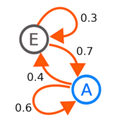
The formalization of the Markov Model [7] shifted the landscape of algorithmic music. With the help of Markov Models, the dice game was extended one step further. Markov Models are built on Markov Chains [8], statistical models of systems that move in between states with the probability of each possible “next” state being dependent solely on the current state of the system. Similar to how the Musicalisches Würfelspiel could be represented via a table, a Markov Chain is encoded via a transitions matrix which contains the probabilities of transitioning between any two possible states within the system. Since Markov Models encode variation in probabilities, they can be trained – the transition matrices can be calculated, and adjusted – based on existing data, as opposed to needing explicitly composed fragments .

In 1958, Iannis Xenakis [9], a Greek-French composer, used a Markov Model to generate two algorithmic pieces of music – Analogique A and Analogique B [10]. Xenakis details his process and the mathematics behind his work in Formalized Music: Thought and Mathematics in Composition . Shortly after, in 1981, David Cope [11], Dickerson Emeritus Professor at the University of California at Santa Cruz, built on Xenakis’s methodology and combined Markov Chains with musical grammars and combinatorics, creating Emmy (Experiments in Musical Intelligence) [12] – a semi-intelligent analysis system that is quite adept at imitating human composers .

The most popular application of Markov Chains is speech recognition (in conjunction with the Viterbi Algorithm). The basic structure of a natural language processing system, and for our purposes, a music system that is built on a Markov Chain is as follows :

1. Take a set (the larger, generally the better) of music data, i.e. compositions.
2. Calculate the log probability of the transition between every two possible pairs of chords. This is accomplished by computing the number of transitions from state A to state B and normalizing this frequency by the total number of transitions out of state A. Note: the transition from state A to state B is independent of the transition from state B to state A.
3. Define a starting state – a first chord. This chord can be randomly generated, or pre-determined.
4. Taking into account the probabilities of transitioning to each possible next state from the current state, randomly pick the next state.
5. Repeat step 4 until the desired length of the composition is reached.

This GitHub code [13] demonstrates this algorithm in practice.

However, although they are intuitive, facile to build, and go a step further than the algorithmic music of the 18th and 19th centuries, Markov Chains are limited in that they can only produce sequences that exist in the original data set(s) that the model was trained on .

A generic RNN cell with labeled inputs, hidden states, and optional outputs. The output of any given node is subsequently the input of the following node. Note, this particular diagram does not contain a cycle, but an RNN possesses the property of non-linearity.

A generic RNN cell that is being trained. The blue vectors are the word embeddings, and the red vectors the hidden states. At every step, the loss function is the negative log probability of the following node's input.

Recurrent Neural Network Cells (RNNs)

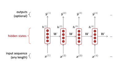
The introduction of Recurrent Neural Networks [14] in 1986, based on the work of American psychologist David Rumelhart [15], drastically changed the field of Algorithmic Composition. The structure of an RNN cell builds on the existing fundamentals from Markov Chains and Neural Networks in general. Both RNN cells and Markov Models attempt to quantify sequential information in data sets, and they work in a very similar manner. Recurrent Neural Networks belong to the family of feedback neural networks with feedback connections.

An RNN cell takes a sequential input of any length (the size of the model does not increase with input length), applies the same weights on each step, allowing for symmetrical input processing, and can optionally produce an output at each step. The information processed at the input and produced at the output is sequential, as opposed to stable. An RNN can be thought of as a series of neural networks connected into a chain.

Much like with Markov Chains, the primary application of RNNs is Language Modelling. The superiority of RNNs over Markov Chains is based on their structure – whereas a current state in a Markov Chain only affects the next possible state (i.e. the probability of any given state occurring is only dependent on the previous state; this is the root of the Markovian assumption), an RNN cell exhibits properties of non-linearity. That is to say, connections between nodes in RNN cells can form cycles, such that the output of a computation at a given node t can eventually factor into the input into that same node t. RNNs are also Turing-Complete , i.e. they can simulate any arbitrary program, provided the relevant set of inputs.

To further dive into the implementation of algorithmic music using a Recurrent Neural Network, let’s take a closer look at the components of music. Any unit of music has three key identifiers: pitch, note, and octave. In brief, the pitch is the degree of highness or lowness of the tone, the note is represented by one of seven letters (A - G), and an octave [16] is an interval between one musical pitch and the same musical pitch with double the frequency. The advantage of RNNs over other types of neural networks with respect to music generation is their usage of sequential data.

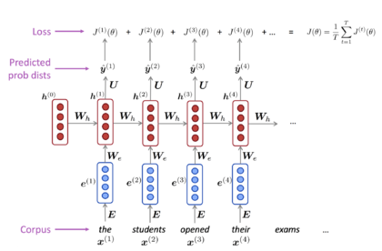
The basic structure of a natural language processing system, and for our purposes, a music system that is built on a Recurrent Neural Network Cell is as follows :

1. Take a set (the larger, generally the better) of music data, i.e. compositions, with each composition represented as a sequence of chords with properties of pitch, note, octave, frequency, and amplitude.
2. Go through the sequence steps and calculate the probability distribution of every possible chord, given the chords occurring so far (computing the output distribution ŷ^(t) for every step t.
3. At every step t, compute the loss function – the cross-entropy between the predicted probability distribution and the true next chord.
4. Take the average of all of the loss functions to compute the overall loss for the entire training set.
5. In practice, computing overall loss using steps 3 and 4 proves too expensive, so practical models use Stochastic Gradient Descent.

This Python tutorial [17] demonstrates this implementation in practice.

However, a major limitation of RNNs is vanishing gradients – the exact short-term coherence that limited the first attempts at creating algorithmic music using RNNs [18] . Specifically, this problem means that the further you go into the network, the lower your gradient is, the harder it is to train your model, and the longer it takes to achieve the final result. The vanishing gradient problem tends to three primary solutions [19]:

1. initialize weights so that the potential for vanishing gradient is minimized;
2. have Echo State Networks that are designed to solve the vanishing gradient problem;
3. have Long Short-Term Memory Networks (LSTMs) – the most popular approach

Using these basic principles, the architecture of an LSTM cell is broken down as follows in the above diagram :

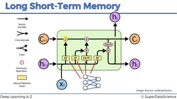
1. Take in the input vector x_t and vector h_t-1 from the previous node
2. Combine the vectors together and plug them into the sigmoid activation function – the output decides if the forget valve should be open, closed, or partially open.
3. Then, the vectors go in parallel through two, layer operations: “tanh” (returns values in the range of -1 to 1) and sigmoid layer operation (returns values in the range 0 to 1). Tanh determines which vector passes through to the memory pipeline. The Sigmoid layer operation determines both with vector passes through to the memory pipeline and also to what extent.
4. Once the vectors have passed through step 3, there is memory flow through the pipeline. If the forget valve is open and the memory valve is closed, then the memory will not change. Otherwise, if the opposite is true, the memory is updated completely.
5. Finally, x_t and h_t-1 combine to determine which part of the memory pipeline becomes the output of this node.

Long Short-Term Memory Cells (LSTMs)

To combat the vanishing gradient problem of RNNs, modern language learning systems and algorithmic music systems implement Long Short-Term Memory cells (LSTMs), first introduced by Sepp Hochreiter in 1997. As the error is propagated throughout the RNN, hidden layers are connected to themselves in times by means of recurrent weights (w_rec). Because the recurrent weight is compounded, we witness the vanishing gradient effect. Numerically speaking, the vanishing gradient problem is present if the recurrent weight achieves a value less than 1 (greater than 1 creates an exploding gradient problem [20]). In a gross oversimplification, Long Short-Term Memory cells make the recurrent weight equal to 1. A brief reminder of the structure of an RNN – the hidden layer receives an input x_t from the input layer at time t, and from itself at time t-1, and it generates an output h_t at time t and also another input for itself at time t+1. To solve the vanishing gradient problem, the structure of an RNN is transformed into an LSTM as follows :

1. Every block has three vector inputs: an input x_t at time t, an output h_t-1 at time point t-1 (this output goes both to the output layer and the hidden layer in the next time point), and the input from a memory cell c_t-1 at time t.
2. Every block also produces two vector outputs: an output h_t and c_t

In 2002, Doug Eck, currently head of the Magenta team at Google Brain, used LSTM cells to create a system that improvised blues music based on a data set of short recordings. The publication is linked here .

Ongoing Projects – MuseNet

Today, there are many ongoing projects in the field of Algorithmic Music. One of particular note is MuseNet . MuseNet is a deep neural network system that generates 4-minute-long musical compositions with up to ten musical instruments. MuseNet implements a large-scale, general-purpose, unsupervised, transformer model , trained to predict the next token in a sequence. The transformer model is based on Recurrent Neural Networks, but takes it a step further, in that it is based solely on attention mechanisms to draw dependencies between input and output. This model allows for significantly more parallelization than previous mechanisms by using stacked self-attention and point-wise, fully connected layers for both the encoder and decoder. The MuseNet system built on the transformer generates quite convincing compositions that indeed sound like they could have been produced by a human. Below are several examples:

Prompt: First 5 notes of Chopin Op. 10, No. 9

Prompt: Jazz Piano-Bass-Drums

Prompt: Bluegrass Piano-Guitar-Bass-Drums

Prompt: First 6 notes of Rachmaninoff

Prompt: Bon Jovi and the first 6 notes of Chopin Op. 27, No. 2

References

- ↑ 1.0 1.1 1.2 Britannica, T. Editors of Encyclopaedia (2019, October 11). Aeolian harp. Encyclopedia Britannica. https://www.britannica.com/art/Aeolian-harp [1]
- ↑ 2.0 2.1 2.2 McDonald, K. (2018, November 13). Neural nets for generating music. Medium. Retrieved November 17, 2022, from https://medium.com/artists-and-machine-intelligence/neural-nets-for-generating-music-f46dffac21c0
- ↑ Xenakis, I., & Kanach, S. (1992). Formalized music: Thought and mathematics in Composition. Pendragon Press. retrieved from https://monoskop.org/images/7/74/Xenakis_Iannis_Formalized_Music_Thought_and_Mathematics_in_Composition.pdf
- ↑ Garcia, C. (2019, September 25). Algorithmic music – David Cope and EMI. CHM. Retrieved November 18, 2022, from https://computerhistory.org/blog/algorithmic-music-david-cope-and-emi/
- ↑ Osipenko, A. (2019, July 7). Markov Chain for Music Generation. Towards Data Science. Retrieved November 18, 2022, from https://towardsdatascience.com/markov-chain-for-music-generation-932ea8a88305
- ↑ Quattrini Li, A., & Pierson, T. (n.d.). PS-5. CS 10: Problem Solving via Object-Oriented Programming. Retrieved November 18, 2022, from https://www.cs.dartmouth.edu/~cs10/schedule.html
- ↑ Goldberg, Y. (n.d.). The unreasonable effectiveness of Character-level Language Models [web log]. Retrieved November 18, 2022, from https://nbviewer.org/gist/yoavg/d76121dfde2618422139.
- ↑ 8.0 8.1 8.2 8.3 See, A. (2022). Lecture 6: Language Models and Recurrent Neural Networks. Natural Language Processing with Deep Learning CS224N/Ling284. Stanford University; Stanford University. Retrieved November 18, 2022, from https://web.stanford.edu/class/cs224n/slides/cs224n-2019-lecture06-rnnlm.pdf.
- ↑ Siegelmann, H. T. (1995). Computation Beyond the Turing Limit. Science, 268, 545–548. Retrieved November 18, 2022, from http://binds.cs.umass.edu/papers/1995_Siegelmann_Science.pdf.
- ↑ 10.0 10.1 SuperDataScience Team. (2018, August 23). Recurrent Neural Networks (RNN) - Long Short Term Memory ( LSTM ) [web log]. Retrieved November 18, 2022, from https://www.superdatascience.com/blogs/recurrent-neural-networks-rnn-long-short-term-memory-lstm/.
- ↑ Hochreiter, S. (1997). LONG SHORT-TERM MEMORY. Neural Computation, 9(8). Retrieved November 18, 2022, from http://www.bioinf.jku.at/publications/older/2604.pdf
- ↑ Eck, D., & Schmidhuber, J. (2002). Finding Temporal Structure in Music: Blues Improvisation with LSTM Recurrent Networks. Neural Networks for Signal Processing XII, Proceedings of the 2002 IEEE Workshop, 747-756. Retrieved November 18, 2022, from http://www.iro.umontreal.ca/~eckdoug/papers/2002_ieee.pdf.
- ↑ Payne, Christine. "MuseNet." OpenAI, 25 Apr. 2019, openai.com/blog/musenet
- ↑ Vaswani, A., Shazeer, N., Parmar, N., Uszkoreit, J., Jones, L., Gomez, A. N., Kaiser, L., & Polosukhin, I. (2017). Attention Is All You Need. arXiv. https://doi.org/10.48550/arXiv.1706.03762